On the Statistics of Interdependent Events

279 In most applications of probability theory, whether in physical, biological or social statistics, only “independent” events are considered. The $n$ individual cases in a statistical series are called “independent” of one another when the chances in each case remain unaffected by the outcome of the other $n-1$. We may, for example, combine all births in Germany during a calendar month into a series and record at each birth whether the newborn child is a boy or a girl. In this respect the individual births are independent of one another; at least, the available numerical material gives no reason to suppose that the chances of a boy being born in the second half of the month are in any way affected by the proportion of boys in the first half — as most readers will believe even without a statistical investigation. But we may also combine into a statistical series all the people who board a railway train in Germany during a calendar month and record for each traveller whether he died during the journey as a result of a railway accident. The individual events in this series are not independent of one another. For the lives of the occupants of the same train are to a high degree “bound together”: the death of one person in a railway accident must be regarded as an extraordinary deterioration in the chances of all his fellow travellers.

The theoretical treatment of events that are not independent would surely be very important for every field in which probability theory is applied, but it is in fact very difficult. An extraordinarily large number of different structures of mutual dependence are conceivable; one must select a structure that, first, represents the structure of the observed series approximately correctly and, second, lends itself sufficiently to calculation for the investigation to be carried through to numerical results.

The present paper investigates a form of probabilistic interdependence [Wahrscheinlichkeitsverkettung] * that broadly represents, for example, the structure of epidemic mortality and of industrial and transport accidents correctly — at any rate much more correctly than the assumption of independent probabilities. Several numerical spot checks, one of which is reported below, strongly support this view. The form of probabilistic interdependence investigated — which might briefly be described as “increase in probability through success” [Chancenvermehrung durch Erfolg] † — is certainly also not unlike the dependence that distributes the individual members of a plant species among the different locations within a uniform natural vegetation cover. The final sections of our paper are devoted to a general investigation, prompted by this observation, of the statistical distribution of point populations [Punktgesamtheiten] in space. Such distributions have a certain interest for physics (radioactive decay, Brownian motion). From the mathematical point of view, one is inevitably led to the problem considered here when one wishes to bring the two simplest and oldest problems of probability theory — repeated draws from an urn with and without replacement of the balls — “under a common denominator”.

The theoretical considerations are due to the second-named author, and the practical execution of the applications to the first-named author.

280 We consider an ordered sequence of quantities $\mathbf{x}_1,\mathbf{x}_2,\ldots,\mathbf{x}_n,\ldots$ subject to chance.1 If the chances on which the outcome of $\mathbf{x}_n$ depends are fixed in advance, unaffected by the outcome of all the others, then $\mathbf{x}_1,\mathbf{x}_2,\ldots,\mathbf{x}_n,\ldots$ are called independent of one another. If the chances of $\mathbf{x}_{n+1}$ are determined by the outcome of $\mathbf{x}_n$ ($n\geq1$), we have a simple chain of quantities, in the terminology of Markoff, to whom we owe a very extensive theory of this simplest case of probabilistic dependence.2 The next simplest case would be that in which the chances of $\mathbf{x}_{n+1}$ are determined by the total result of the preceding chance outcomes, that is, by the value taken by the sum $\mathbf{x}_1+\mathbf{x}_2+\cdots+\mathbf{x}_n$. Unfortunately, a general theory of this kind of dependence is not yet available; a special case will be treated here and first illustrated by the urn scheme.

At the beginning of the game an urn contains $R$ red and $S$ black balls, $R+S=N$ balls in all. A ball is drawn from the urn, and in place of the ball drawn, $1+\Delta$ balls of the same colour are put into the urn. Another ball is then drawn and the same operation repeated. After the $n$th draw the urn therefore contains $N+n\Delta$ balls. If $r$ red and $s$ black balls ($r+s=n$) have been drawn in the first $n$ draws, the urn contains $R+r\Delta$ red and $S+s\Delta$ black balls, and the probabilities of drawing a red or a black ball respectively on the $(n+1)$th draw are

$$\frac{R+r\Delta}{N+n\Delta}=\frac{\varrho+r\delta}{1+n\delta},\qquad \frac{S+s\Delta}{N+n\Delta}=\frac{\sigma+s\delta}{1+n\delta}.\qquad(1)$$

Here, for brevity, we have put

$$\frac{R}{N}=\varrho,\qquad \frac{S}{N}=\sigma,\qquad\frac{\Delta}{N}=\delta.\qquad(2)$$

For $\Delta=0$ we have the familiar problem of balls drawn with replacement, and for $\Delta=-1$ that of balls drawn without replacement.

We can express this more abstractly as follows: the random variables $\mathbf{x}_1,\mathbf{x}_2,\ldots,\mathbf{x}_n,\ldots$ can take only two values, 1 and 0. Let the probability that $\mathbf{x}_1=1$ (a red draw) be $\varrho$, and the probability that $\mathbf{x}_1=0$ (a black draw) be $\sigma$, with $\varrho+\sigma=1$. Let

$$\begin{aligned} &\frac{\varrho+(\mathbf{x}_1+\mathbf{x}_2+\cdots+\mathbf{x}_n)\delta}{1+n\delta},\\[0.6em] &\frac{\sigma+(n-\mathbf{x}_1-\mathbf{x}_2-\cdots-\mathbf{x}_n)\delta}{1+n\delta}.\qquad(3) \end{aligned}$$

be the probabilities that $\mathbf{x}_{n+1}=1$ and $\mathbf{x}_{n+1}=0$, respectively. If we put

$$\mathbf{x}_1+\mathbf{x}_2+\cdots+\mathbf{x}_n=r,\qquad s=n-r,\qquad(4)$$

then formulae (1) and (3) are identical. If $\delta>0$, there is an increase in probability through success and a decrease in probability through failure; when $\delta<0$ the reverse holds. Thus, when $\delta>0$, both success and failure are “contagious”. The value $\delta=0$ gives the classical, simplest case of independent events. When $\delta\geq0$ the sequence of quantities $\mathbf{x}_1,\mathbf{x}_2,\ldots$ can be continued indefinitely; when $\delta<0$, only as long as $1+n\delta>0$.*

What is the probability that $\mathbf{x}_1+\mathbf{x}_2+\cdots+\mathbf{x}_n=r$? (The possible values of $r$ are $0,1,2,\ldots,n$.) In other words, what is the probability, under the stated conditions, of drawing $r$ red and $s=n-r$ black balls from the urn in $n$ draws? By the multiplication rule for probabilities, the probability that $$\mathbf{x}_1=1,\ \mathbf{x}_2=1,\ldots,\mathbf{x}_r=1,\quad \mathbf{x}_{r+1}=0,\ldots,\mathbf{x}_{r+s}=0$$ is

$$\begin{aligned} &\frac{\varrho}{1}\frac{\varrho+\delta}{1+\delta}\frac{\varrho+2\delta}{1+2\delta}\cdots \frac{\varrho+(r-1)\delta}{1+(r-1)\delta}\\[0.5em] &\qquad{}\times\frac{\sigma}{1+r\delta}\frac{\sigma+\delta}{1+(r+1)\delta}\cdots \frac{\sigma+(s-1)\delta}{1+(n-1)\delta}.\qquad(5) \end{aligned}$$

The probability that $r$ specified members of $\mathbf{x}_1,\mathbf{x}_2,\ldots,\mathbf{x}_n$ take the value 1 and the remaining $s$ take the value 0 is again given by (5). For if 281 one forms the corresponding product according to (3), one again obtains $n$ fractions whose denominators are the same as those in (5), while the numerators merely occur in a different order. The calculation therefore amounts simply to a permutation of the factors in the numerator (not in the denominator!). From $n$ elements one can select $r$ in $\binom nr$ ways; hence the required probability is

$$p_{r,s}=\frac{n!}{r!s!} \frac{\begin{gathered} \varrho(\varrho+\delta)\cdots(\varrho+(r-1)\delta)\\[-0.2em] {}\times\sigma(\sigma+\delta)\cdots(\sigma+(s-1)\delta) \end{gathered}} {1(1+\delta)(1+2\delta)\cdots(1+(n-1)\delta)}.\qquad(6)$$

We now calculate the mathematical expectation of $\mathbf{r}(\mathbf{r}-1)(\mathbf{r}-2)\cdots(\mathbf{r}-k+1)$. Denote the quantity to be calculated by $\langle\mathbf{r}(\mathbf{r}-1)\cdots(\mathbf{r}-k+1)\rangle$.1 According to (6), $$\begin{aligned} &\langle\mathbf{r}(\mathbf{r}-1)\cdots(\mathbf{r}-k+1)\rangle\\[0.4em] &\quad=\sum_{r=0}^n r(r-1)\cdots(r-k+1)p_{r,n-r}\\[0.8em] &\quad=\dfrac{ \displaystyle\sum_{r+s=n}\left[\begin{aligned} &r(r-1)\cdots(r-k+1)\\[0.4em] &\quad{}\times\dfrac{\frac{\varrho}{\delta}(\frac{\varrho}{\delta}+1)\cdots(\frac{\varrho}{\delta}+r-1)}{r!}\\[0.6em] &\quad{}\times\dfrac{\frac{\sigma}{\delta}(\frac{\sigma}{\delta}+1)\cdots(\frac{\sigma}{\delta}+s-1)}{s!} \end{aligned}\right] }{\dfrac{\frac1\delta(\frac1\delta+1)\cdots(\frac1\delta+n-1)}{n!}}. \end{aligned}$$

Thus, in the sum in the numerator, $r=0,1,2,\ldots,n$ and $s=n-r$ are to be taken.* The numerator is the coefficient of $z^n$ in the product of the two series $$\begin{aligned} &\left[\sum_{r=0}^{\infty}r(r-1)\cdots(r-k+1) \frac{\frac{\varrho}{\delta}(\frac{\varrho}{\delta}+1)\cdots(\frac{\varrho}{\delta}+r-1)}{r!}z^r\right]\\[0.5em] &\quad{}\times\left[\sum_{s=0}^{\infty}\frac{\frac{\sigma}{\delta}(\frac{\sigma}{\delta}+1)\cdots(\frac{\sigma}{\delta}+s-1)}{s!}z^s\right]\\[0.8em] &=\left(z^k\frac{d^k}{dz^k}(1-z)^{-\varrho/\delta}\right)(1-z)^{-\sigma/\delta}\\[0.6em] &=z^k\frac{\varrho}{\delta}\left(\frac{\varrho}{\delta}+1\right)\cdots\left(\frac{\varrho}{\delta}+k-1\right)\\ &\qquad{}\times(1-z)^{-\varrho/\delta-k}(1-z)^{-\sigma/\delta}\\[0.6em] &=\frac{\varrho}{\delta}\left(\frac{\varrho}{\delta}+1\right)\cdots\left(\frac{\varrho}{\delta}+k-1\right)z^k(1-z)^{-1/\delta-k}\\[0.6em] &=\frac{\varrho}{\delta}\left(\frac{\varrho}{\delta}+1\right)\cdots\left(\frac{\varrho}{\delta}+k-1\right)\\[0.2em] &\qquad{}\times\sum_{n=k}^{\infty}\frac{(\frac1\delta+k)(\frac1\delta+k+1)\cdots(\frac1\delta+k+n-k-1)}{(n-k)!}z^n. \end{aligned}$$

Hence $$\begin{aligned} &\langle\mathbf{r}(\mathbf{r}-1)\cdots(\mathbf{r}-k+1)\rangle\\[0.5em] &\quad=\dfrac{\begin{gathered} \frac{\varrho}{\delta}(\frac{\varrho}{\delta}+1)\cdots(\frac{\varrho}{\delta}+k-1)\\[0.4em] {}\times(\frac1\delta+k)(\frac1\delta+k+1)\cdots(\frac1\delta+n-1)\frac1{(n-k)!} \end{gathered}} {\frac1\delta(\frac1\delta+1)\cdots(\frac1\delta+n-1)\frac1{n!}}, \end{aligned}$$

$$\begin{aligned} &\langle\mathbf{r}(\mathbf{r}-1)\cdots(\mathbf{r}-k+1)\rangle\\[0.4em] &\quad=\frac{\varrho(\varrho+\delta)(\varrho+2\delta)\cdots(\varrho+(k-1)\delta)} {1(1+\delta)(1+2\delta)\cdots(1+(k-1)\delta)}\\[0.4em] &\qquad{}\times n(n-1)\cdots(n-k+1).\qquad(7) \end{aligned}$$

Formula (7) can also be obtained by other, more combinatorial considerations. In particular, for $k=1,2$, (7) gives the expected value of $\mathbf{r}$ and the variance about this expectation [Quadrat der mittleren Abweichung]:†

$$\langle\mathbf{r}\rangle=\varrho n.\qquad(8)$$

$$\begin{aligned} \langle(\mathbf{r}-\langle\mathbf{r}\rangle)^2\rangle &=\langle\mathbf{r}^2\rangle-\langle\mathbf{r}\rangle^2\\[0.3em] &=\langle\mathbf{r}(\mathbf{r}-1)\rangle+\langle\mathbf{r}\rangle-\langle\mathbf{r}\rangle^2\\[0.5em] &=\frac{\varrho(\varrho+\delta)}{1(1+\delta)}n(n-1)+n\varrho-n^2\varrho^2\\[0.5em] &=n\varrho(1-\varrho)\frac{1+n\delta}{1+\delta}.\qquad(9) \end{aligned}$$

For $\delta=0$, or for $\delta=-1/N$, $\varrho=R/N$, $\sigma=S/N$ — compare (2) — these yield the familiar classical results, which may serve as a check.

We turn to circumstances in which the number of observed cases $n$ is very large, but $\varrho$ is so small — that is, the characteristic with probability $\varrho$ is so rare — that the expected number $\langle\mathbf{r}\rangle=\varrho n$ is only small. For example, let $n$ be the number of people who begin a railway journey within a month, and $\varrho$ the probability that the journey undertaken ends in a fatal accident. Put

$$n\varrho=h,\qquad n\delta=d>0,\qquad(10)$$

282 and suppose $h$ and $d$ to be moderate and $n$ very large; or, in an appropriate mathematical abstraction, hold $h$ and $d$ fixed and let $n$ tend to infinity. We first calculate the limiting value of the probability $p_{0,n}$. According to (6), $$\begin{aligned} p_{0,n}&=\frac{\sigma(\sigma+\delta)\cdots(\sigma+(n-1)\delta)}{1(1+\delta)\cdots(1+(n-1)\delta)}\\ &=\left(1-\frac\varrho1\right)\left(1-\frac\varrho{1+\delta}\right)\left(1-\frac\varrho{1+2\delta}\right)\cdots \left(1-\frac\varrho{1+(n-1)\delta}\right). \end{aligned}$$

Substituting, according to (10),

$$\varrho=\frac hn,\qquad\sigma=1-\frac hn,\qquad\delta=\frac dn,\qquad(11)$$

we obtain $$p_{0,n}=\left(1-\frac hn\right)\left(1-\frac h{n+d}\right)\cdots\left(1-\frac h{n+(n-1)d}\right),$$ $$\begin{aligned} \lg p_{0,n}={}&-\left(\frac hn+\frac h{n+d}+\cdots+\frac h{n+(n-1)d}\right)\\ &-\frac12\left[\left(\frac hn\right)^2+\cdots+\left(\frac h{n+(n-1)d}\right)^2\right]-\cdots, \end{aligned}$$

$$\lg p_{0,n}=-\frac hd\left(\frac dn+\frac dn\frac1{1+d/n}+\cdots+\frac dn\frac1{1+(n-1)d/n}\right)-R_n.\quad(12)$$

The remainder $R_n$ becomes infinitesimal as $n\to\infty$; it is of order $1/n$, as is easily verified. The expression in brackets on the right of (12) is to be regarded as a sum of $n$ rectangles with base $d/n$. If they are placed side by side on the abscissa axis so that their bases fill the interval between abscissae 0 and $d$, their upper left corners lie on the curve $y=1/(1+x)$. Hence* $$\begin{aligned} \lim_{n\to\infty}\lg p_{0,n} &=-\frac hd\lim_{n\to\infty}\sum_{\nu=1}^{n}\frac dn\frac1{1+(\nu-1)d/n}\\[0.5em] &=-\frac hd\int_0^d\frac{dx}{1+x}\\[0.5em] &=-\frac hd\lg(1+d). \end{aligned}$$

$$\lim_{n\to\infty}p_{0,n}=(1+d)^{-h/d}=P_0.\qquad(13)$$

From (6) and (11) it follows that $$\begin{aligned} p_{r,n-r}&=p_{0,n}\frac{n(n-1)\cdots(n-r+1)}{1\cdot2\cdots r}\\[0.3em] &\quad{}\times\frac{\varrho}{\sigma+(n-1)\delta}\frac{\varrho+\delta}{\sigma+(n-2)\delta}\cdots \frac{\varrho+(r-1)\delta}{\sigma+(n-r)\delta}\\[0.8em] &=p_{0,n}\frac{\begin{gathered} (1-\frac1n)(1-\frac2n)\cdots(1-\frac{r-1}n)\\[-0.1em] {}\times h(h+d)\cdots(h+(r-1)d) \end{gathered}} {r!\,(1+d-\frac{h+d}n)(1+d-\frac{h+2d}n)\cdots(1+d-\frac{h+rd}n)}. \end{aligned}$$

For fixed $r$, this formula, together with (13), gives $$\lim_{n\to\infty}p_{r,n-r}=(1+d)^{-h/d}\frac1{r!}\frac h{1+d}\frac{h+d}{1+d}\cdots\frac{h+(r-1)d}{1+d}$$

$$=\frac1{r!}h(h+d)(h+2d)\cdots(h+(r-1)d)(1+d)^{-h/d-r}=P_r.\quad(14)$$

As a check on formula (14), we calculate the sum of the limiting probabilities $P_0,P_1,P_2,\ldots,P_r,\ldots$. We have $$\begin{aligned} \sum_{r=0}^{\infty}P_r &=(1+d)^{-h/d}\sum_{r=0}^{\infty} \frac{\frac hd(\frac hd+1)\cdots(\frac hd+r-1)}{1\cdot2\cdots r}\left(\frac d{1+d}\right)^r\\ &=(1+d)^{-h/d}\left(1-\frac d{1+d}\right)^{-h/d}=1. \end{aligned}$$

For a further check on (14), we calculate the expectation $$\begin{aligned} &\langle\mathbf{r}(\mathbf{r}-1)\cdots(\mathbf{r}-k+1)\rangle\\[0.4em] &=\sum_{r=0}^{\infty}r(r-1)\cdots(r-k+1)P_r\\[0.6em] &=(1+d)^{-h/d}\\[0.2em] &\quad{}\times\left[z^k\frac{d^k}{dz^k}\sum_{r=0}^{\infty} \frac{\frac hd(\frac hd+1)\cdots(\frac hd+r-1)}{1\cdot2\cdots r}z^r\right]_{z=d/(1+d)}\\[0.8em] &=(1+d)^{-h/d}\left(\frac d{1+d}\right)^k\\[0.3em] &\quad{}\times\frac hd\left(\frac hd+1\right)\cdots\left(\frac hd+k-1\right) \left(1-\frac d{1+d}\right)^{-h/d-k}. \end{aligned}$$

$$\langle\mathbf{r}(\mathbf{r}-1)\cdots(\mathbf{r}-k+1)\rangle=h(h+d)(h+2d)\cdots(h+(k-1)d).\quad(15)$$

We could also have obtained the same result directly from (7) by passing to the limit. In particular, either from (15) or by passing to the limit in (8) and (9), we obtain the following values for the expectation $\langle\mathbf{r}\rangle$ and the variance 283 about it:

$$\langle\mathbf{r}\rangle=h.\qquad(16)$$

$$\langle(\mathbf{r}-h)^2\rangle=h(1+d).\qquad(17)$$

So far we have considered the case $d>0$, that is, the case of an increase in probability through success. For $d=0$ we have $$\lim_{d\to0}P_0=\lim_{d\to0}(1+d)^{-h/d}=e^{-h}=P_0^*,$$ and, generally, compare (14),

$$\lim_{d\to0}P_r=\frac{h^r e^{-h}}{r!}=P_r^*.\qquad(18)$$

Thus, for $d=0$, the formulae derived include the familiar case of independent rare events, discovered by Poisson and recognised in its significance for statistics by L. von Bortkiewicz.1

The probabilities $P_0,P_1,P_2,\ldots,P_r,\ldots$ given by formula (14) arise, in brief, from the following probabilistic structure: the body of observations is very large, the characteristic under investigation is very rare, and the individual observed cases are linked in such a way that the more strongly the characteristic is represented in one part of the observations, the more strongly it is also to be expected in the remainder. The observed cases might, for instance, be the deaths in a particular country within a month, and the particular characteristic under investigation death from a rare epidemic disease such as smallpox or cholera. The registration of an especially large number of smallpox cases in the first half of the month prejudges what is to be expected in the second half of the month in the same direction. Railway accidents or industrial accidents, for example those resulting from an explosion, spread, statistically speaking, in much the same way as a contagious disease, since they generally claim several lives. We may expect the statistical figures for phenomena of this kind to agree qualitatively with the course of the probabilities $P_0,P_1,P_2,\ldots,P_r,\ldots$.

Now for a quantitative test! Take, for example, the deaths from smallpox in Switzerland during the years 1877–1900, that is, during 288 months; compare Table 1, original p. 285. There were 1,584 such deaths in all, giving a monthly average of 5.5. If we put

$$h=5.5,\qquad(19)$$

we can calculate the probabilities $P_0^*,P_1^*,\ldots$ from formula (18) ($P_0^*,P_1^*,\ldots,P_r^*,\ldots$ correspond to independent rare events). The quantity $288P_r^*$ is the expected (theoretical) number, among the 288 observed months, of months in which exactly $r$ deaths should occur; compare column III of Table 1. The actual number of these months is in column II of Table 1. Column VI of Table 1 contains the numbers $288(P_0^*+P_1^*+\cdots+P_r^*)=288\sum_{\nu=0}^rP_\nu^*$, set beside the corresponding observed numbers in column V. Thus, at the intersection of column V and row $r$ (where $r=0,1,2,\ldots$) stands the number of months, among the 288 observed, in which no more than $r$ deaths of the kind in question occurred. The disagreement between the theory that assumes the independence of the individual cases and leads to the probabilities $P_0^*,P_1^*,\ldots,P_r^*,\ldots$ and the available facts is apparent either from a comparison of columns II and III, or from one of columns V and VI, or, finally, from the following consideration. If the events are independent, the variance ought to be $h$ (compare formula (17) for $d=0$; in our case $h=5.5$). Multiplying $(r-5.5)^2$ by the number of months in which exactly $r$ deaths occurred (compare column II, row $r$), summing from $r=0$ to $r=60$, and dividing the resulting sum by 287, that is, the total number of months minus 1, gives 83.5888, a value considerably greater than 5.5.*

284 To test the theory of an increase in probability through success against this case, we use formula (17) to determine $d$ from the equation $$h(1+d)=83.5888$$ (the calculation of the number 83.5888 has just been explained). We obtain

$$d=14.20.\qquad(20)$$

With the numerical values (19) and (20), we calculate the probabilities $P_0,P_1,P_2,\ldots$ according to formula (14). Comparing columns II and IV, and still more columns V and VII, of Table 1 shows, at first sight, an entirely satisfactory quantitative agreement between the theoretical expected numbers in IV and VII and the corresponding observed numbers in II and V.

Of course, the result that better agreement was obtained with the $P_r$ than with the $P_r^*$ could also be attributed to the circumstance that the $P_r^*$ contain only one adjustable parameter, namely $h$, whereas the $P_r$ contain two, namely $h$ and $d$. We incline, however, to the view that the better agreement arises not merely from this external circumstance but rather from the much better agreement of the probabilistic picture with reality when an increase in probability through success is assumed than when independence of the cases is assumed. Tests of the theory against other statistical material gave, in part, even more favourable results. The first-named author will publish the details elsewhere.

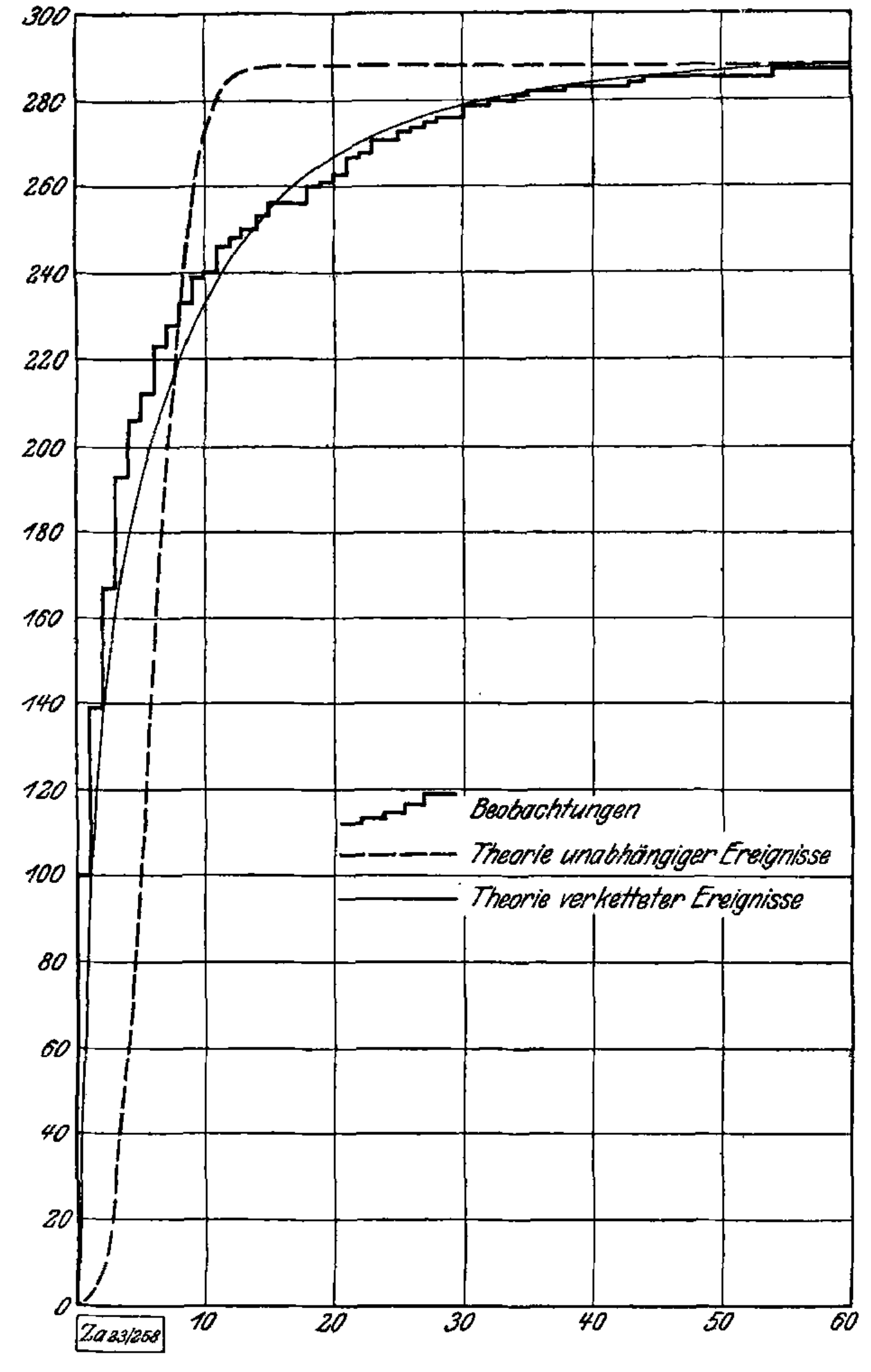
Comparison of theory and observation in the Swiss smallpox statistics. (The ordinate at abscissa $x$ gives the number of months in which the number of deaths is less than $x$ or equal to $x$.)

Graph key, translated from the original: stepped line — observations; dashed line — theory of independent events; continuous curve — theory of interdependent events.

Whether the space in question is one-, two- or three-dimensional makes only an insignificant difference to the following discussion. For definiteness, let us consider the two-dimensional case: the points are distributed in a plane.

Let a plane region $F$ of area $f$ be given. By saying that a point $P$ is scattered over the region $F$, we mean the following: if $F'$ is any subregion of $F$, with area $f'$, the probability that the point $P$ lies in the subregion $F'$ is $f'/f$. It is now clear what is meant by several points being scattered over $F$ independently of one another. If $r+\nu$ points are scattered independently over $F$, the probability that $r$ of the $r+\nu$ points fall in the subregion $F'$ and $\nu$ outside it is

$$\binom{r+\nu}{\nu}\left(\frac{f'}f\right)^r\left(1-\frac{f'}f\right)^\nu.\qquad(21)$$

To characterise the distribution of a point population in a plane in terms of probability theory, one must specify the probability $W(r,F)$ that exactly $r$ points of the population lie within a region $F$ (with $r$ and $F$ arbitrary). Suppose the distribution is uniform [gleichmäßig], that is, $W(r,F)$ depends neither on the position nor on the shape of the region, but only on its area $f$: $W(r,F)=W_r(f)$.† Thus, to characterise a uniform distribution of points in the plane, one must specify the probabilities

$$W_0(f),W_1(f),W_2(f),\ldots,W_r(f),\ldots.\qquad(22)$$

The functions (22) are subject to the conditions

$$W_r(f)\geq0\quad\text{for }r=0,1,2,3,\ldots;\quad f>0,\qquad(\mathrm{I})$$

$$W_0(f)+W_1(f)+W_2(f)+\cdots+W_r(f)+\cdots=1.\qquad(\mathrm{II})$$

The distribution of a point population shall be called stable [stabil], in the probabilistic sense, if purely random disturbances cannot alter anything essential in it. More precisely: the stability of the distribution of a point population consists in the fact that the overall statistical picture remains unchanged when the points of the population lying within any region $F$ are removed from $F$ and scattered back over $F$ independently of one another.‡

Outside $F$, removing and scattering back the points lying in $F$ obviously changes nothing; we therefore need only consider what it changes in any subregion $F'$ of $F$. Let the distribution be assumed uniform from the outset and specified by the probabilities (22), satisfying (I) and (II). As above, denote the areas of $F$ and $F'$ by $f$ and $f'$.

Before the points were removed from $F$, the probability that exactly $r$ points lay in $F'$ was $W_r(f')$.

For exactly $r$ points to lie in $F'$ after removal and scattering back, $r+\nu$ points must have been present in $F$ originally, with $\nu\geq0$. The probability that $r+\nu$ points were in $F$ is $W_{r+\nu}(f)$; the probability that exactly $r$ of these $r+\nu$ fall in $F'$ when scattered back is given by (21). Since $\nu$ may be $0,1,2,3,\ldots$, the probability that exactly $r$ points lie in $f'$ after scattering back is $$\sum_{\nu=0}^{\infty}W_{r+\nu}(f)\binom{r+\nu}{\nu}\left(\frac{f'}f\right)^r\left(1-\frac{f'}f\right)^\nu.$$

287 Thus, the stability of the distribution specified by the probabilities (22) is expressed by the equation

$$\begin{gathered} W_r(f')=\sum_{\nu=0}^{\infty}W_{r+\nu}(f)\binom{r+\nu}{\nu}\left(\frac{f'}f\right)^r\left(1-\frac{f'}f\right)^\nu,\qquad(\mathrm{III})\\ 0<f'\leq f,\qquad r=0,1,2,3,\ldots. \end{gathered}$$

To find the functions (22) satisfying conditions (I), (II) and (III), put

$$W_0(f)+W_1(f)z+W_2(f)z^2+\cdots=\Phi(f,z).\qquad(23)$$

The series (23) has positive coefficients, compare (I), and converges for $z=1$, compare (II), and therefore throughout $f>0$, $|z|\leq1$; $z$ is regarded as a complex variable. Multiply (III) by $z^r$ and sum over $r=0,1,2,\ldots$; this gives

$$\begin{aligned} &\sum_{r=0}^{\infty}W_r(f')z^r\\[0.4em] &\quad=\sum_{r=0}^{\infty}\sum_{\nu=0}^{\infty}z^rW_{r+\nu}(f) \binom{r+\nu}{\nu}\left(\frac{f'}f\right)^r\left(1-\frac{f'}f\right)^\nu.\qquad(24) \end{aligned}$$

For brevity, put

$$\frac{f'}f=x,\qquad0<x\leq1.\qquad(25)$$

From (24) we obtain $$\begin{aligned} &\Phi(fx,z)\\[0.4em] &=\sum_{r=0}^{\infty}\sum_{\nu=0}^{\infty} \frac{(r+\nu)(r+\nu-1)\cdots(r+1)}{\nu!}W_{r+\nu}(f)(zx)^r(1-x)^\nu\\ &=\sum_{\nu=0}^{\infty}\frac{(1-x)^\nu}{\nu!}\sum_{r=0}^{\infty} W_{r+\nu}(f)(r+\nu)(r+\nu-1)\cdots(r+1)(zx)^r\\ &=\sum_{\nu=0}^{\infty}\frac{(1-x)^\nu}{\nu!}\Phi^{(\nu)}(f,zx), \end{aligned}$$ in accordance with (23), where $\Phi^{(\nu)}(x,y)=\partial^\nu\Phi/\partial y^\nu$. Thus

$$\Phi(fx,z)=\Phi(f,zx+1-x).\qquad(26)$$

Put $\Phi(1,u+1)=\Psi(u)$.

For the variables $f,x,z$, substitute either $1,f,z$, or $f,1/f,1+(z-1)f$; the first choice is appropriate when $f\leq1$, and the second when $f\geq1$, in view of the inequality in (25). In both cases we obtain

$$\Phi(f,z)=\Psi(fz-f).\qquad(27)$$

Substituting the power-series expansion (23) for $\Phi(f,z)$ in (27) gives, by Maclaurin’s formula,

$$\sum_{r=0}^{\infty}W_r(f)z^r=\sum_{r=0}^{\infty}\frac{\Psi^{(r)}(-f)f^r}{r!}z^r,\qquad(28)$$

and, by comparison of coefficients,

$$W_r(f)=\frac{\Psi^{(r)}(-f)f^r}{r!}\quad(r=0,1,2,\ldots).\qquad(29)$$

From the validity of the power-series expansion (28) in the domain $f>0$, $|z|\leq1$, and from conditions (I) and (II), we finally reach the following result: if the distribution of the point population defined by the probabilities (22) is to be stable, those probabilities are given by equation (29), where $\Psi(u)$ is a function analytic in the half-plane $\operatorname{Re}(u)<0$, all of whose derivatives are real and positive for real negative values of $u$; furthermore, $\lim_{u\to0}\Psi(u)=1$ as $u$ approaches the point 0 from the left half-plane.

As $u$ tends to 0 through negative values, $\Psi'(u)$ always increases, since $\Psi''(u)>0$ for $u<0$.

288 Let

$$\lim_{u\to0}\Psi'(u)=D\qquad(30)$$

be finite. Then $D>0$, and by (29) $$\begin{aligned} \sum_{r=0}^{\infty}rW_r(f)&=\sum_{r=1}^{\infty}\frac{rf^r\Psi^{(r)}(-f)}{r!}\\[0.5em] &=f\sum_{m=0}^{\infty}\frac{f^m\Psi^{(1+m)}(-f)}{m!}\\[0.5em] &=f\Psi'(0)=fD. \end{aligned}$$ The quantity $D$ is the average number of points in the population per unit area — in short, the density [Dichte] of the point population.

To say that the individual parts of the point population are independent of one another means that the chances of the distribution in each region are unaffected by the outcome of the distribution in the other regions. Let the distribution be uniform and specified by the probabilities (22). Consider two regions $F_1$ and $F_2$, of areas $f_1$ and $f_2$ respectively, which together make up a region $F$ of area $f_1+f_2=f$. If the individual parts of the point population are independent of one another, the probability that exactly $n$ points lie in $f_2$ remains $W_n(f_2)$, regardless of whether 0, 1, 2, 3, … points lie in the neighbouring region $f_1$. Consequently, the probability that $m$ points lie in $f_1$ and $n$ points in $f_2$ is $W_m(f_1)W_n(f_2)$, and the probability that a total of $r$ points lie in $f$ is

$$\begin{aligned} &W_0(f_1)W_r(f_2)+W_1(f_1)W_{r-1}(f_2)+\cdots+W_r(f_1)W_0(f_2)\\[0.4em] &\qquad=W_r(f_1+f_2).\qquad(31) \end{aligned}$$

For the function $\Phi(f,z)$ defined in (23), this gives the relation

$$\Phi(f_1+f_2,z)=\Phi(f_1,z)\Phi(f_2,z).\qquad(32)$$

If arbitrary subpopulations are independent of one another, $f_1$ and $f_2$ can be chosen arbitrarily. As is well known, the validity of (32) for every pair $f_1,f_2$ with $f_1>0$, $f_2>0$ entails the equation

$$\Phi(f,z)=e^{\varphi(z)f},\qquad(33)$$